Module Basics: Sheet Music Analysis with music21
- Tutorial Jupyter_SheetMusic_Basics_Introduction_music21 (Jupyter-Notebook; html preview)
- Tutorial Jupyter_SheetMusic_Basics_Part1_Visualisation (Jupyter-Notebook; html preview)
- Tutorial Jupyter_SheetMusic_Basics_Part2_Statistics (Jupyter-Notebook; html preview)
This page provides basic information for the module Basics Sheet Music Analysis with music 21. Various examples introduces into working with music21 and Jupyter Notebooks, visualizing of music scores and statistical queries.
The requirements for running Jupyter Notebooks in the browser are the installation of Anaconda respectively Miniconda and of the score editor MuseScore. Detailed installation instructions and introductory tutorials can be found here:
- Installation Jupyter Notebook, Anaconda und Miniconda
- Tutorial Jupyter Notebook
- Installation MuseScore
- Tutorial MusicXML in depth
After successful installation, please save the three Jupyter notebook tutorials (see above) to your computer (right click → save target as). Choose as location the path of the default working folder you get to when starting Jupyter notebooks (usually 'c:/users/ name' - where 'name' is specifically assigned to your computer). Create a folder „Analysis“ there, where you then store all notebooks.
| Attention: Jupyter notebooks have the file extension '.ipynb'. Unfortunately, some operating systems change the ending to ´.txt´ and, then, the files get assigned to a text editor. In this case please change the ending back to ´.ipynb´, otherwise the Jupyter Notebooks cannot be opened. |
| The html versions can only be read, not executed or modified; they are for preliminary information only! |
Afterwards you should briefly familiarise yourself with the concept of Jupyter notebooks and the basic commands in music21 as well as adapt some settings for music21 to your local device.
This will be helped by the
- Tutorial Jupyter_SheetMusic_Basics_Introduction_music21 (Jupyter-Notebook; html preview)
| A quick and uncomplicated introduction to the possibilities of computer-aided music analysis with music21 is offered by the Interactive Music Analysis. Here you can get to know the various statistical queries by selecting options, without having to get involved in the command syntax of music21 and how the Jupyter notebooks work. (The installation of Anaconda or Miniconda as well as MuseScore.)is required). |
Following the Basics module, you can turn to the tutorials in the Advanced Notes module:
- Tutorial Jupyter_SheetMusic_Advanced_Part1_Josquin (Jupyter-Notebook; html preview)
- Tutorial Jupyter_SheetMusic_Advanced_Part2_Beethoven (Jupyter-Notebook; html preview)
Tutorial 1: Visualisation of sheet music
Jupyter_SheetMusic_Basics_Part1_Visualisation (Jupyter-Notebook; html preview)
Usually, music notation on which musical analysis is usually based on are playing instructions for the musicians. This is called prescriptive notation. In contrast, musical structures which are to be described in the analysis - and as far as possible as they are sounded.
From prescriptive notation the American musicologist Charles Seeger distinguished a descriptive notation with which an attempt is made to show musical structures graphically. The purpose of these visualisations is not to perform music, but to get as good an impression as possible of its tonal structures and textures, such as the fabric of the various voices over time and in pitch space.
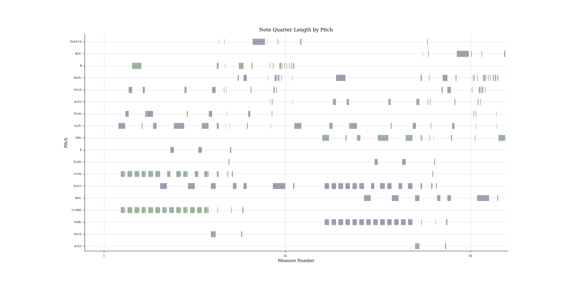
A simple descriptive notation is the two-dimensional arrangement of all played notes: The y-axis corresponds to absolute pitch, the x-axis to time. Different instruments can be colored differently. This depiction is called piano roll representation because the rolls for player pianos were punched according to this pattern.
The following piano roll visualisations is from the Tutorial Basics Noten 1 to show how sheet music is displayed in an intuitive way.
| Note: You can display piano rolls very clearly in the Sonic Visualiser and listen to them with MIDI sounds at the same time. A number of piano rolls are listed in the subcorpus of the sheet music database and can be downloaded there. Detailed instructions on how to proceed and how you could generate piano rolls from score files can be found here. |
Music21 also offers the possibility to automatically generate piano reductions of music scores (chordify-command). This facilitates for example harmonic analysis.
The tutorial also explains a few other useful features of music21, including the selection of excerpts (measures) and voices.
Tutorial 2: Statistical queries of musical characteristics
Jupyter_SheetMusic_Basics_Part1_Visualisation (Jupyter-Notebook; html preview)
The music21 commands presented in the Jupyter notebooks can first be used to query the number of notes (total or per voice), measures, and information about ambitus (total and per voice).
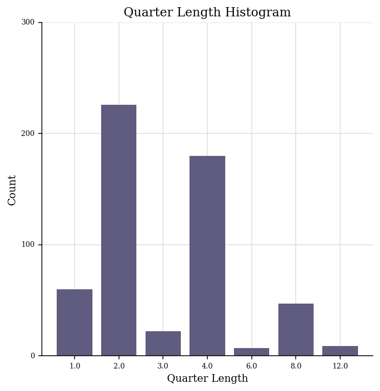
By examining frequencies, you can get a first overview of the simplicity and uniformity or the variety and complexity of a composition. For example, is only the diatonic tone stock used in the composition, or are there also many chromatic tones? Do the individual voices progress mainly in small interval steps or are there (also) large leaps? Are there only a few different note durations or a big variety of note values?
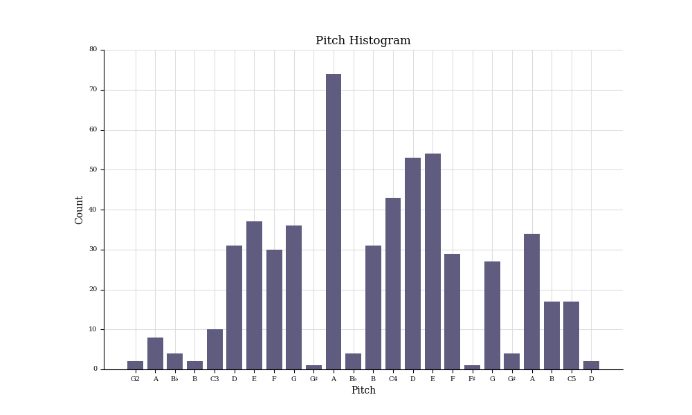
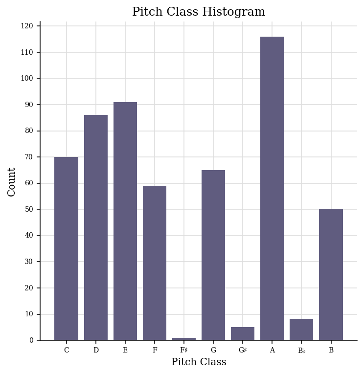
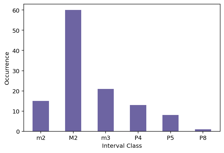
These questions are answered by histograms showing frequency distributions (=bar charts) and spreadsheets. You can determine and display frequencies of the following parameters or variables (among others) by the use of simple commands:
Frequencies of pitches can be queried per score file and per voice. A distinction is made between different octave positions.
Frequencies of the twelve pitch classes - per voice and in total. No distinction is made between different octave positions!
The English pitch designations are used:
C C#/Db D D#/Eb E F F#/Gb G G#/Ab A A#/Bb B C
Frequencies of interval steps or jumps within a voice.
Attention: This is just possible for monophonic voices!
The following interval names are used:
 Perfect unison= 0
 Minor second= m2
 Major second= M2
 Minor third= m3
 Major third= M3
 Perfect fourth= P4
 Etc.
Frequencies of note durations / note values
Note values are counted as multiples or parts of a quarter note:
 Quarter = 1
 Eighths = 0.5
 Half = 2
 Etc.
Metric Weight
Music21 offers a way to determine the metric weight (the metric accent) of each note (1.0 = highest weight, 0.5 = middle weight, 0.25 lower weight etc.) by the beat-strength-command and to calculate the frequencies of the individual weights or accent levels. This allows to understand how clearly or unambiguously a meter is established in the music.
The metrical accents follow the following weighting for the common time signatures (each for a sequence of eighth notes):
4/4: [1.0, 0.125, 0.25, 0.125, 0.5, 0.125, 0.25, 0.125]
 2/4: [1.0, 0.25, 0.5, 0.25]
 3/4: [1.0, 0.25, 0.5, 0.25, 0.5, 0.25]
 6/8: [[1.0, 0.25, 0.25, 0.5, 0.25, 0.25]
 9/8: [1.0, 0.25, 0.25, 0.5, 0.25, 0.25, 0.5, 0.25, 0.25]
 2/2: [1.0, 0.125, 0.25, 0.125, 0.5, 0.125, 0.25, 0.125]

 1.0 = highest weight, 0.5 = medium weight, 0.25 lower weight etc.
Two-dimensional frequency distributions
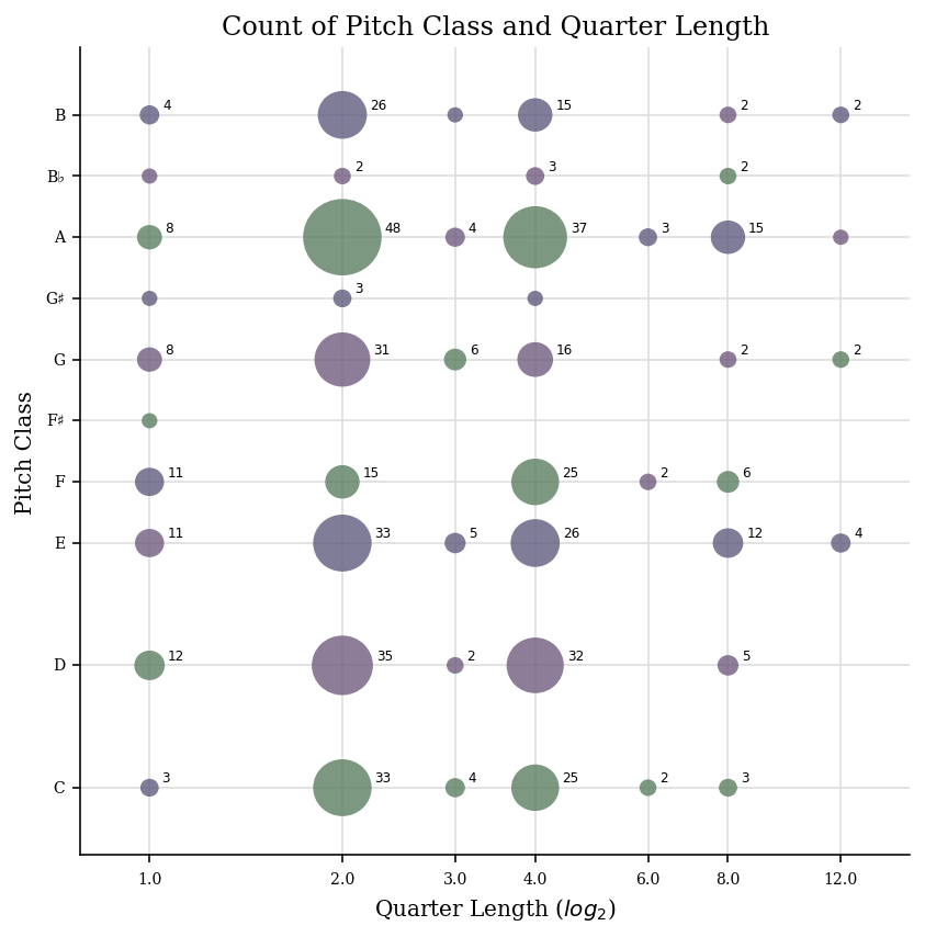
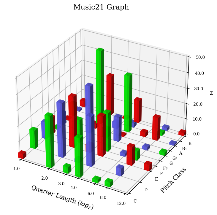
In addition, two of the mentioned musical parameters can be displayed in so-called two-dimensional frequency distributions, i.e. in dependence on each other, e.g. the frequencies of the individual pitches coupled in each case with certain duration values (quarter, eighth etc.). The two-dimensional frequency distributions can be displayed as scatter plots or 3D plots. With music21, the following parameters can be related to each other:
- • Frequency of note duration related to pitch and pitch class
- • Frequency of metric positions, respectively metric weight related to pitch and pitch class
All statistical queries can be applied to
- individual movements and excerpts of compositions
- on complete compositions as well as
- several compositions in comparison!
In this way, individual compositions, but also corpora of compositions can be analyzed.
Furthermore, it is possible to export the frequency distributions as so-called csv files („csv“ =„comma-seperated values“). The csv format can be opened and read by spreadsheet software such as Excel, among others. In this way, the data can be processed externally, which can be particularly useful for corpus studies.
